library(yahtsee)
#> Loading required package: tsibble
#>
#> Attaching package: 'tsibble'
#> The following objects are masked from 'package:base':
#>
#>     intersect, setdiff, union
library(ggplot2)
library(dplyr)
#>
#> Attaching package: 'dplyr'
#> The following objects are masked from 'package:stats':
#>
#>     filter, lag
#> The following objects are masked from 'package:base':
#>
#>     intersect, setdiff, setequal, union
The data
For this model we are going to fit a very simple model using some summarised data from the malariaAtlas R package, malaria_africa_ts:
malaria_africa_ts
#> # A tsibble: 1,046 x 15 [1D]
#> # Key:       country [46]
#>    who_region who_subregion country date       month_num positive examined
#>    <fct>      <fct>         <fct>   <date>         <dbl>    <dbl>    <int>
#>  1 AFRO       AFRO-W        Angola  1989-06-01       120     15.8       50
#>  2 AFRO       AFRO-W        Angola  2005-11-01       372     82        111
#>  3 AFRO       AFRO-W        Angola  2006-04-01       300    102        197
#>  4 AFRO       AFRO-W        Angola  2006-11-01       384     41        347
#>  5 AFRO       AFRO-W        Angola  2006-12-01       396    173        734
#>  6 AFRO       AFRO-W        Angola  2007-01-01       276    216        828
#>  7 AFRO       AFRO-W        Angola  2007-02-01       288     42         71
#>  8 AFRO       AFRO-W        Angola  2007-03-01       300    119        448
#>  9 AFRO       AFRO-W        Angola  2011-01-01       324      1        239
#> 10 AFRO       AFRO-W        Angola  2011-02-01       336    148       1132
#> # … with 1,036 more rows, and 8 more variables: pr <dbl>, avg_lower_age <dbl>,
#> #   continent_id <fct>, country_id <fct>, year <int>, month <int>,
#> #   avg_upper_age <dbl>, species <fct>
This data has the following features we are interested in:
- hierarchical structure (countries within who subregion, within region)
- Positive rate measurements recorded over time for these areas (positive rate given by the number of positive cases divided by the number of cases examined).
(Note that we are still getting some more covariates for this data.)
tsibble data
This data is a tsibble (the “ts” is pronounced like the end of “bats”).
This is a speical time series aware table, that knows what elements identify the individual time components, in this case, country, and what the time index is, in this case, date.
We use a tsibble because it stores this time (referred to as an “index”) and group (referred to as a “key”) information, which we can use inside our modelling software.
Modelling
Let’s say we want to model the pr over time. Here is a plot of the pr over time, where each line is a country, and facets represent the different who subregions:
ggplot(malaria_africa_ts,
       aes(x = date,
           y = pr,
           group = country,
           colour = who_subregion)) +
  geom_line() +
  facet_wrap(~who_subregion) +
  theme(legend.position = "none")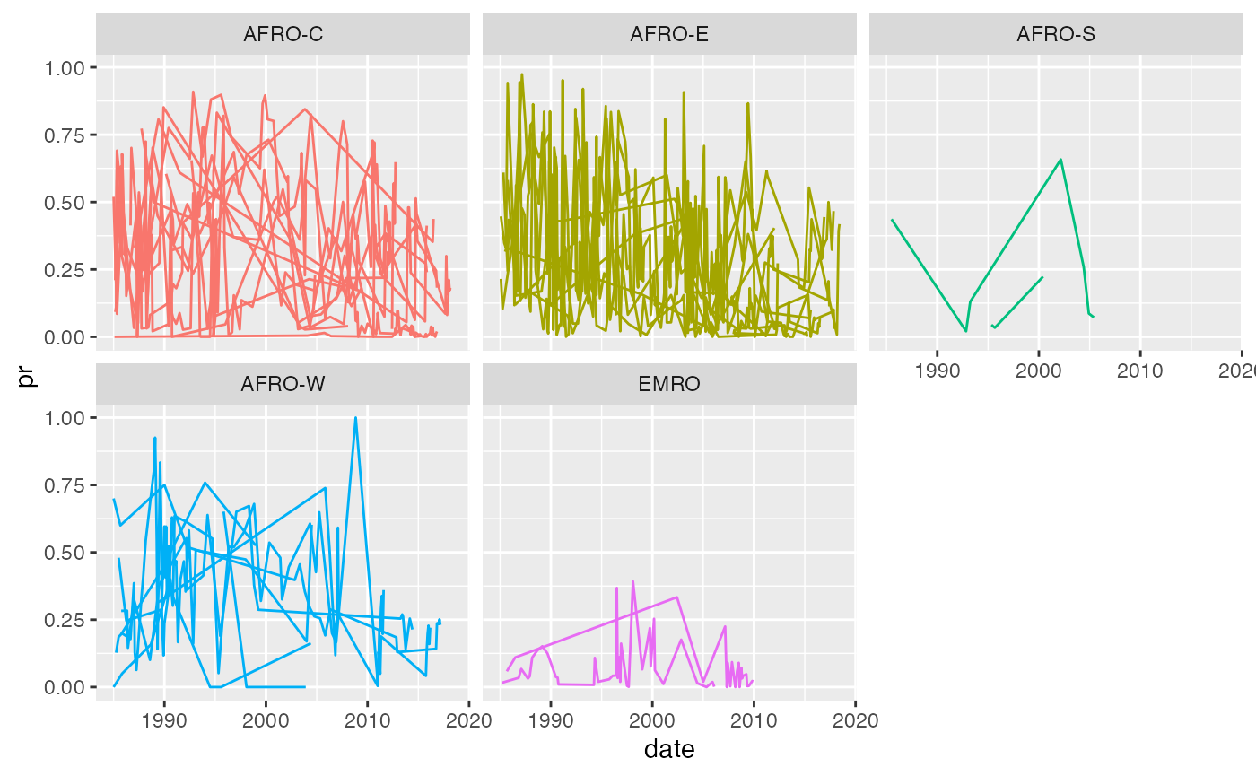
Let’s create a simple model that has fixed effect of lower age. We add a AR1 process for each of these subregions using the hts() component in the formula. Here, the inputs arethe levels of hierarchy, in order of decreasing size:
pr ~ avg_lower_age + hts(who_region, who_subregion, country)We then provide the data, likelihood family (in this case “gaussian”, but all INLA likelihoods are available).
We specify the time component at the moment using the special_index argument, but this will be removed later once we resolve a couple of bugs to do with the data.
m <- fit_hts(
    # inputs are  the levels of hierarchy, in order of decreasing size
  formula = pr ~ avg_lower_age + hts(who_region, who_subregion, country),
  .data = malaria_africa_ts,
  family = "gaussian",
  special_index = month_num
)
The equivalent model fitted with inlabru would look like the following:
inlabru::bru(
formula = pr ~ avg_lower_age + Intercept +
  who_region(month_num,
             model = "ar1",
             group = .who_region_id,
             constr = FALSE) +
  who_subregion(month_num,
                model = "ar1",
                group = .who_subregion_id,
                constr = FALSE) +
  country(month_num,
          model = "ar1",
          group = .country_id,
          constr = FALSE),
    family = "gaussian",
    data = malaria_africa_ts,
    options = list(
      control.compute = list(config = TRUE),
      control.predictor = list(compute = TRUE, link = 1)
      )
      )
Here are some of the extra considerations that need to be made:
- What to name the random effects (who_region, who_subregion, country)
- Specifying the time component of the ar1 process
- repeating the “ar1” component for each random effect
- The
groupargument requires a special index variable of a group to be made (.who_subregion_id) - Additional options passed to
inlabruin options to help get the appropriate data back.
Proposed workflow
The proposed workflow of this type of model is as follows:
- Specify data as a
tsibbleobject:
library(tsibble)
malaria_africa_ts <- as_tsibble(x = malaria_africa,
                                key = country,
index = date)- Fit the model, parsing the hierarchy structure
model_hts <- fit_hts(
    # inputs are  the levels of hierarchy, in order of decreasing size
  formula = pr ~ avg_lower_age + hts(who_region, who_subregion, country),
  .data = malaria_africa_ts,
  family = "gaussian"
)- Perform diagnostics
diagnostics(model_hts)
autoplot(model_hts)- Make prediction data
date_range <- clock::date_build(2019, 2, 1:5)
date_range
#> [1] "2019-02-01" "2019-02-02" "2019-02-03" "2019-02-04" "2019-02-05"
countries <- c("Ethiopia", "Tanzania")
countries
#> [1] "Ethiopia" "Tanzania"
df_pred <- prediction_data(
  model_data = malaria_africa_ts,
  key = countries,
  index = date_range
)

df_pred
#> # A tsibble: 10 x 2 [1D]
#> # Key:       country [2]
#>    country  date
#>    <chr>    <date>
#>  1 Ethiopia 2019-02-01
#>  2 Ethiopia 2019-02-02
#>  3 Ethiopia 2019-02-03
#>  4 Ethiopia 2019-02-04
#>  5 Ethiopia 2019-02-05
#>  6 Tanzania 2019-02-01
#>  7 Tanzania 2019-02-02
#>  8 Tanzania 2019-02-03
#>  9 Tanzania 2019-02-04
#> 10 Tanzania 2019-02-05- Post hoc prediction from the model to add uncertainty information
# post-hoc prediction function - with options for presenting the uncertainty
pred <- predict(m, df_pred, se.fit = TRUE)